
S, E, I, R, H, Q, V, D… and others
As I mentioned in the previous article, the simplest epidemiological models are the “compartmentalized” models, in which the population is divided into groups representative of the development of the epidemic. The origin of these models dates back to the beginning of the 20th century, the generally cited reference article being (Kermack & McKendrick, 1927), although this article is in fact much more general.
The concept of “compartment” is easy to understand when compared to the daily statistics on the COVID-19 pandemic: number of cases, deaths, recoveries, and in a more detailed way (for example on geodes.santepubliquefrance.fr): number of hospitalizations, intensive care admissions, etc. This categorization corresponds to the schematic stages of development of the patients’ health status, and therefore to the “compartments” used in the simplified models.
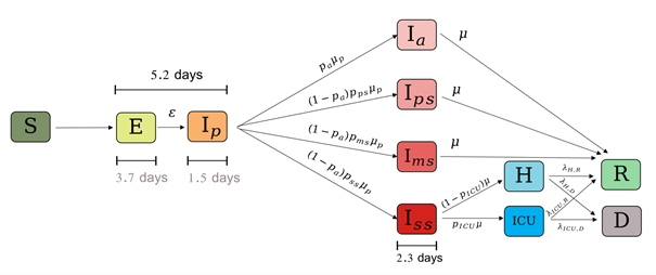
The compartments are generally identified by letters, the grouping of which gives the name of the model. One of the simplest models is the SIR model: in English, these are the initials Susceptible, Infected and Recovered or Removed (depending on whether or not the possibility of death is considered). The number and type of compartments depend on the epidemic to be modeled and the level of detail desired. For example, INSERM (Di Domenico & al., 2020) uses for COVID-19 a model with three age classes and 11 compartments, for most of the subclasses of compartment I (see figure below).
Presentation of the SIR model
“Exponential growth”, “flattening the curve”, “epidemic peak”, “herd immunity”, or “reproductive number (or rate)”… These expressions, frequently heard or read in the media, implicitly refer to compartmentalized epidemiological models. To know what they mean, it is essential to go through the equation of a model, and the SIR model is simple enough to understand the logic of the phenomena studied. I will pose the model directly, giving some “hands-on” explanations and leaving aside the sordid mathematical details, and then discuss the implications of this approach in relation to current events.
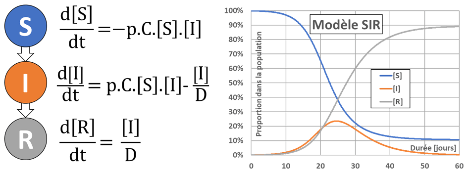
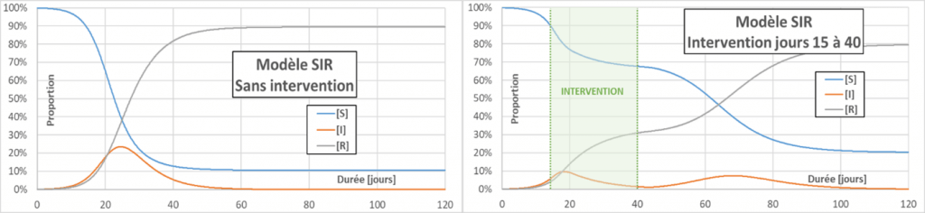
The following image shows the three compartments used (S for Healthy or Susceptible, I for Infected and R for Remitted or Recovered, no death is considered for the moment), the evolution equations for the proportions of the compartments’ numbers noted [S], [I] and [R], and the results of a typical simulation. We note that in this model the R individuals are immune and therefore cannot be re-infected.
Change in the number of employees in the compartments
Proportion of healthy individuals [S]
The proportion [S] of healthy individuals is decreasing. The rate of decrease is the product of the total number of daily contacts between healthy and infected individuals C.[S][I] by the probability p that a contact results in transmission of infection; C being the average number of daily contacts per individual. In order to limit contamination, one can therefore seek to reduce p, C, or possibly [I].
Preventive quarantine:
The “stage 1” of epidemic management aims at slowing down the introduction of the infectious disease into the national territory. The aim is to reduce [I] (closing borders, identifying chains of transmission and quarantining people who are infected or returning from a risk area, etc.).
Barrier gestures: Wearing a mask and gloves, frequent hand washing, keeping a safe distance, putting up protective screens… All these measures aim to reduce the probability p of being infected during contact, and thus contribute to curbing the spread of the epidemic.
Social Distanciation:
The “stage 2” aims to slow down the spread of an epidemic on the national territory. To do this, actions to reduce the number of daily contacts C are implemented: closure of schools, restaurants, and more generally ERPs (establishments receiving the public), limitation of transport, stopping visits to the most vulnerable people, etc. and finally general confinement of the population.
Proportion of individuals cured, or “handed over” [R]
The proportion [R] of individuals recovered is only increasing, by progressive healing of the people in compartment I. The evolution equation is constructed from the mean time to recovery D, and the proportion of individuals cured each day is estimated to be given by [I]/D. This simplifying hypothesis (which is equivalent to saying that the duration of healing follows an exponential law of probability), which is generally ignored, is nevertheless fraught with consequences because this law of probability is not adapted to the problem. On the other hand, it fits easily into the equation of the SIR model (pragmatism of the modeler!).
Basic reproduction number: the product p.C.D corresponds to the total number of contaminations that an infected individual can cause during the entire time of his infection (product of the daily number of contacts C by the number of days in the infectious state D and by the probability of transmitting the infection during contact p). This is the famous “R0” or “basic reproductive number”, which is much talked about. This basic number depends on the country (age pyramid…), on the cultural notion of pimping (Marret, 2020), on social habits (kissing, shaking hands…), etc.
Proportion of infected individuals [I]
The proportion of individuals infected at a given time varies according to the two previous proportions, since [I]=1-[S]-[R] according to the constant population hypothesis. The two contributions to this evolution are antagonistic: on the one hand [I] will increase by contamination of healthy people (S->I passage) and on the other hand it will decrease by healing of infected people (I->R passage).
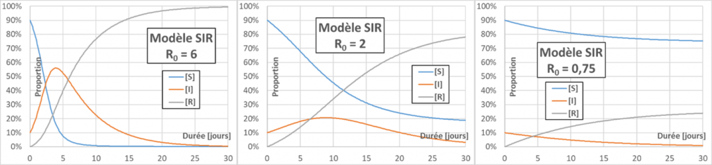
Epidemic peak: at the beginning of an epidemic [S] is about 1, and the sign of d[I]/dt is given by the sign of (p.C.D-1), i.e. R0-1. If R0 is greater than one, each infected person has time to infect more than one during his or her infectious period, the epidemic will spread (snowball effect), and an epidemic peak is observed. Otherwise, the epidemic extinguishes itself (figure below – for better readability the initial rate of infected people is set at 10%). The higher the R0, the higher the epidemic peak (maximum of [I]) will be.
Exponential growth: In the early days of the epidemic, we saw that [S]~1. The evolutionary relation of [I] is then of the form d[I]/dt=k.[I]. This relation is easily integrated to obtain explicitly [I]=[I]0.exp(k.t), where [I]0 is the initial fraction of infected population and exp is the exponential function. If R0>1, k is positive and the evolution of [I] at short times therefore shows “exponential growth”.
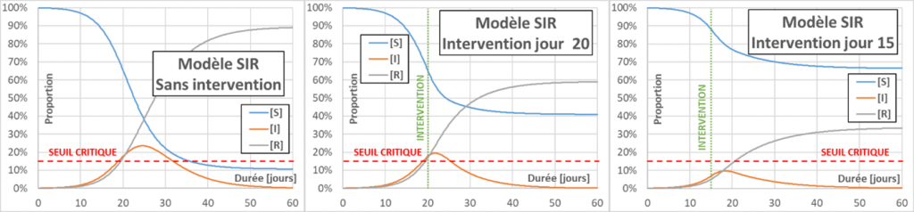
Flattening the curve: Actions aimed at decreasing p, C or D (for the latter, by drug treatment for example) will decrease the effective reproduction number Reff (contrary to what we often hear – even in the mouth of a minister – the R0 does not change). When Reff decreases, the infection curve flattens, the peak of infection is less and the total number of infected people also decreases. The main interest in flattening the curve is to limit serious cases, to avoid overloading the emergency services. In the following figure, a reference case (without intervention) is compared with two cases aiming to decrease Reff to a value of 0.75. In one case the intervention occurs on day 20, and in the other on day 15. The figure also shows a (fictitious) critical threshold for emergency department overload. The value of taking very early action can be seen.
Collective immunity: The effective reproductive Reff number also decreases, in the course of an epidemic, with the proportion of healthy people [S]. If p, C and D remain unchanged, when can an epidemic “naturally” decrease? The sign of (p.C.[S]-1/D) again gives us the answer: The epidemic will decrease when [S] becomes less than 1/R0. At this point, the proportion of people who have been infected is the sum of [I] (those who are still infected) and [R] (those who are cured). Since [S]+[I]+[R]=1, the previous stopping criterion also translates into [I]+[R]>1-1/R0. This is “herd immunity”, which is easily understood: the risk of contact between healthy and infected people decreases when there are very few healthy people left; the many healed people “buffer” between the other two categories.
Second wave: Containment does not pretend to solve the problem of an epidemic, but to save time on the development of vaccines and treatments as well as on the adaptation of workplaces, and of course not to overburden emergency services by “flattening the curve”. When containment is released, new cases will emerge, as shown in the figure below: this is the “second wave”. In addition to the decrease in epidemic peaks compared to a situation without intervention, a greater proportion of individuals who have never been infected is also observed in the end.
Stop-and-go : Dernier slogan médiatique en date, le “stop-and-go” désigne une stratégie de gestion de l’épidémie basée sur l’alternance entre périodes de confinement et périodes de reprise d’activité, afin de multiplier les « petits pics » et d’étaler dans le temps la survenue de nouveaux cas. Comme pour le confinement simple, il s’agit essentiellement de gagner du temps par rapport à l’élaboration des vaccins et traitements, en essayant de maintenir à flot l’activité économique du pays.
General reflections on the model and its results
Limitations of compartment models
The first limitation of compartmentalized models is the homogeneity of the population studied and the inert-individual contacts. In these models, an individual has the same probability of meeting any other individual in the population, but our contacts do not take place in this way: we create privileged relationships – and therefore possible contacts – through multiple networks (our neighborhood, our work, the associations in which we participate, the businesses we frequent…) and not in an undifferentiated way. Moreover, the average number of contacts varies greatly between individuals (according to age, temperament…), but also according to the time of the year or by participation in certain exceptional events (attending a soccer match, being invited to a wedding, etc.). More refined approaches use “contact matrices” associated with various transmission probabilities. These probabilities of transmission are not constant and should, for an infected person, change over time (for example, the notion of “viral load” could be used).
The second limitation is the absence of a spatial dimension. What is obvious in an epidemic is the presence of geographically localized “infectious foci” (or “clusters”), which will lead to a very different development of the epidemic depending on the country, region or city. In compartmentalized models, each individual can be in contact with any other, without any notion of distance or local population density, which is of course not the case in “real” life. Taking into account a spatial dimension can be done in many ways, but it is not easy to integrate in a compartmentalized model. The article (Yeghikyan, 2020) illustrates these first two points well.
The third limitation is a wobbly consideration of the temporal dimension. We have seen that the representation of the duration before healing was not adapted. All the temporal phases of the more complex compartmental models (duration between resuscitation and death, between infection and consultation, between start of treatment and cure, between contamination and start of transmission, etc.) are represented in the same way. More appropriate solutions exist, but are much more complex to implement: for example, “delay” functions can be used, for example by formalizing for the SIR model a link between [R](t) and [I](t-d), according to a more adequate probability law for d.
The fourth limit is the deterministic character of the resolution. A simulation starting from the same starting conditions will necessarily lead to the same result, and the uncertainties on these results will not appear clearly, giving the impression that the results of the model have the character of absolute truth. However, it is quite easy to switch to stochastic resolution by varying the initial parameters and conditions and running several hundred simulations instead of a single simulation (Monte-Carlo type approach). Instead of well-defined curves, an average curve will appear surrounded by a zone of probable variation, for example a 95% confidence interval. In some cases, this zone of uncertainty is so large that the model is of no practical interest anymore… The article (Gonçalves, 2020) deals in particular with this point, and as for the previous one, Python codes are provided to be able to reproduce the results and test variants.
Difficulties of the parameterization
The SIR model includes only two parameters: the p.C. product (which can be individualized if necessary) and the duration D. Unfortunately, an epidemic does not arrive with its identity card, and the values of its characteristic parameters have to be found by processing the observable epidemic propagation data.
What do we have for COVID-19? A good knowledge of the evolution curve of [I] would give us at least R0-1, but official accounting excludes de facto asymptomatic or pauci-symptomatic cases, since these cases do not lead to hospitalization or a visit to the doctor. Moreover, the actual method of counting varies over time: for France, the initial data came from hospitals only, then partial data (mainly deaths) from HPAE were added, and then data from city medicine (consultations with a symptomatic table evoking COVID-19), at the risk of also counting “canada-dry” cases of other lung diseases: it looks like COVID, it has the symptoms of COVID, but it is not COVID…
As you have understood, we cannot rely on death data either, for the same reasons as above (not to mention that the mortality rate depends on many other parameters, and it is therefore difficult to trace back to [I]…). Recent information suggests that several thousand deaths at home are also due to COVID and have not been accounted for. INSEE is beginning to use information on excess mortality compared to previous years, but the associated statistical treatment is extremely complex because the cause of death is not indicated, and the excess mortality due to COVID is partially offset by other phenomena, such as the decrease in traffic accidents, among others.
The only way to really know the proportion of people affected by COVID-19 is to carry out very large scale tests in order to better understand the response levels of individuals to the infection as well. The death rate of infected individuals could also be better known, since the observed deaths would be reduced to the total number of infections and not only to those infections that resulted in hospitalization.
But then, what’s the point?
It is clear that the SIR model and its different variants are too simple to predict the fate of the infection with a correct reliability. Adding parameters and compartments amplifies the difficulties associated with parameterization, and such a simple model cannot be better than the data that supports it, data whose collection is too uncertain to serve as an absolute reference. The variability of the parameters published for COVID-19 in the literature also illustrates the complexity of the problem .
If such a model can only be calibrated at the end of an epidemic (or by periodically revising the values of the parameters to make them match the observed data as closely as possible), and if it therefore has no predictive value, what good can it do?
First of all, these models allow qualitative comparisons of scenarios: what would happen if contacts were significantly reduced (by 25%, 50%, etc.), if the containment period were extended by 10 days or a month, etc.? This could also make it possible to communicate to the population about the benefits of barrier gestures, social distancing, etc., even if it is necessary to first “popularize” certain concepts. This is not a great success in my opinion for the moment, and we are essentially subjected to the anxiety-provoking accounting of new cases and deaths, without any attempt at contextualization and explanation, not to mention a lot of unreliable and contradictory information…
In conclusion: how can an epidemic be stopped?
In the end, this is still the most important thing: how can it end?
Herd immunity – a false good idea: Under the optimistic assumptions of post-infection acquired immunity (we will come back to this later), an R0 of 2 and a mortality rate for infected individuals of 0.5%, the threshold of immunity to COVID-19 would be reached when at least 50% of the population has acquired the virus. For the French population (67 million people), this would lead to more than 167,000 deaths. With less optimistic assumptions (R0=2.5; 1% mortality), the 400,000 deaths would easily be exceeded, and even more in the event of saturation of the emergency services (because the mortality rate would be much higher). So no, clearly herd immunity is not a solution!
Vaccination: To put it simply, vaccination means going directly from compartment S to compartment R, without going through the “disease” phase (which avoids deaths). The minimum effective vaccination rate is therefore the same as the threshold for herd immunity, i.e. 1-1/R0. Vaccination, if possible, would be effective against COVID-19.
Spontaneous remission: By analogy with the influenza virus, and because known coronaviruses also appear to be sensitive to exposure to dry air, some scientists believe that the epidemic could self-limit in the summer (a few weeks ago, this was referred to as “spring”). This does not mean that the pandemic would stop for good, but that it could become seasonal, or take root endemically in our territories. In short, we will live with it for a long time to come…
What if immunity is not acquired?
An infection leads the organism to generate antibodies (their detection is the operating principle of serological tests). One can hope that people who are seropositive for Coronavirus will be definitively immune to it (compartment R), but this is by no means a certainty. Does immunity depend on the initial level of infection? Is it long-lasting? Would it be valid against mutations of the virus? The scientific community is currently unable to answer these crucial questions.
In the worst case, if there is no immunity, the SIR model is reduced to an SI model: compartment S behaves like the pierced barrel of Danaïdes : As the compartment fills up by the “return” of infected individuals I into susceptible individuals S (and no longer “healthy” in this case), it empties through new infections that transform the individuals S into I. Needless to say in this case everyone would eventually catch the disease (and even several times over the years).
This doubt about immunity to COVID also raises questions about the possibility of developing a fully effective vaccine. In addition to the initial difficulty (as no vaccine has been developed so far for a coronavirus), there is also uncertainty about the feasibility of a vaccine and questions about possible mutations in COVID-19, which would lead to a permanent work of adaptation of the vaccine (like Sisyphus and his rock, to change the mythological metaphor). A vaccine, even an imperfect one, that would limit the possibility of developing severe forms of the disease, would already be very good news… which is not expected before (at best) mid-2021.
Until then, we can at least hope for the development of treatments which, if administered early enough, would reduce the risk of death in case of illness… We therefore rely a lot on researchers, and of course and always on caregivers, many thanks to them!
To go further :
The articles and websites cited in the text are referenced below. I would also like to mention the excellent site https://www.3blue1brown.com/ and its YouTube channel, which presents extremely well-made popular science videos, even for very complex domains (the author even provides the Python code that allows to create one’s own animations). Concerning our subject, I highly recommend the videos “Exponential Growth and Epidemics” and especially “Simulating an epidemic”, in which the themes I have tackled find a very original illustration.
Di Domenico L., Pullano G., Sabbatini C.E., Boëlle P.-Y., Colizza V. ; Expected impact of lockdown in Île-de-France and possible exit strategies; Report #9; www.epicx-lab.com/covid-19.html.
Gonçalves B., Article medium, 2020 : https://medium.com/data-for-science/epidemic-modeling-101-or-why-your-covid19-exponential-fits-are-wrong-97aa50c55f8
Kermack W.O. and McKendrick A.G.; “A contribution to the Mathematical Theory of Epidemics”; Proc. R. Soc. Lond. A, 115 ; pp. 700-721; (1927).
Marret J.-L.; COVID-19 : la distance sociale (confinement et proximité : une approche par les sciences sociales) ; Note n°09/20, Fondation pour la Recherche Stratégique.
Yeghikyan G., Article towardsdatascience, 2020 : https://towardsdatascience.com/modelling-the-coronavirus-epidemic-spreading-in-a-city-with-python-babd14d82fa2